Archive for Storage

RAID Levels

mirror-from-IKEA

What is RAID?

RAID stands for Redundant Array of Inexpensive (Independent) Disks. Data is distributed across the drives in one of several ways called “RAID levels”, depending on what level of redundancy and performance is required.

RAID Concepts

  • Striping
  • Mirroring
  • Parity or Error Correction
  • Hardware or Software RAID

RAID Levels

0,1,5 and 10 are the most commonly used RAID Levels

  • RAID 0

RAID_0.svg

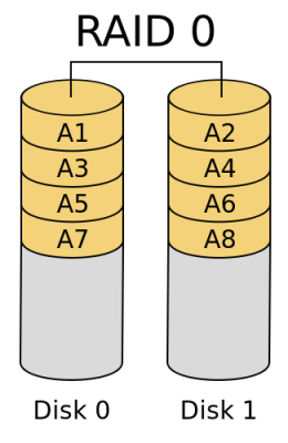
RAID 0 (block-level striping without parity or mirroring) has no (or zero) redundancy. It provides improved performance and additional storage but no fault tolerance. Hence simple stripe sets are normally referred to as RAID 0. Any drive failure destroys the array, and the likelihood of failure increases with more drives in the array. A single drive failure destroys the entire array because when data is written to a RAID 0 volume, the data is broken into fragments called blocks. The number of blocks is dictated by the stripe size, which is a configuration parameter of the array. The blocks are written to their respective drives simultaneously on the same sector. This allows smaller sections of the entire chunk of data to be read off each drive in parallel, increasing bandwidth. RAID 0 does not implement error checking, so any read error is uncorrectable. More drives in the array means higher bandwidth, but greater risk of data loss.

  • RAID 1

RAID_1.svg

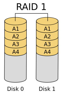
In RAID 1 (mirroring without parity or striping), data is written identically to two drives, thereby producing a “mirrored set”; the read request is serviced by either of the two drives containing the requested data, whichever one involves least seek time plus rotational latency. Similarly, a write request updates the stripes of both drives. The write performance depends on the slower of the two writes (i.e., the one that involves larger seek time and rotational latency); at least two drives are required to constitute such an array. While more constituent drives may be employed, many implementations deal with a maximum of only two. The array continues to operate as long as at least one drive is functioning. With appropriate operating system support, there can be increased read performance as data can be read off any of the drives in the array, and only a minimal write performance reduction; implementing RAID 1 with a separate controller for each drive in order to perform simultaneous reads (and writes) is sometimes called “multiplexing” (or “duplexing” when there are only two drives)

When the workload is write intensive you want to use RAID 1 or RAID 1+0

  • RAID 5

RAID_5.svg

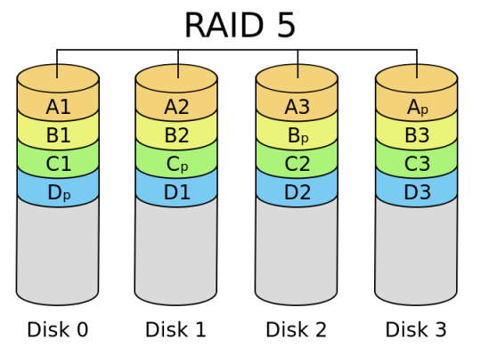
RAID 5 (block-level striping with distributed parity) distributes parity along with the data and requires all drives but one to be present to operate; the array is not destroyed by a single drive failure. Upon drive failure, any subsequent reads can be calculated from the distributed parity such that the drive failure is masked from the end user. However, a single drive failure results in reduced performance of the entire array until the failed drive has been replaced and the associated data rebuilt, because each block of the failed disk needs to be reconstructed by reading all other disks i.e. the parity and other data blocks of a RAID stripe. RAID 5 requires at least three disks. Best cost effective option providing both performance and redundancy. Use this for DB that is heavily read oriented. Write operations will be dependent on the RAID Controller used due to the need to calculate the parity data and write it across all the disks

When your workloads are read intensive it is best to use RAID 5 or RAID 6 and especially for web servers where most of the transactions are read

Don’t use RAID 5 for heavy write environments such as Database servers

  • RAID 10 or 1+0 (Stripe of Mirrors)

RAID_10

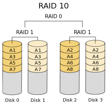
In RAID 10 (mirroring and striping), data is written in stripes across primary disks that have been mirrored to the secondary disks. A typical RAID 10 configuration consists of four drives, two for striping and two for mirroring. A RAID 10 configuration takes the best concepts of RAID 0 and RAID 1, and combines them to provide better performance along with the reliability of parity without actually having parity as with RAID 5 and RAID 6. RAID 10 is often referred to as RAID 1+0 (mirrored+striped) This is the recommended option for any mission critical applications (especially databases) and requires a minimum of 4 disks. Performance on both RAID 10 and RAID 01 will be the same.

  • RAID 01 (Mirror of Stripes)

raid01

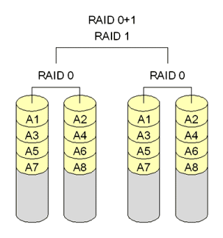
RAID 01 is also called as RAID 0+1. It requires a minimum of 3 disks. But in most cases this will be implemented as minimum of 4 disks. Imagine  two groups of 3 disks. For example, if you have total of 6 disks, create 2 groups. Group 1 has 3 disks and Group 2 has 3 disks.
Within the group, the data is striped. i.e In the Group 1 which contains three disks, the 1st block will be written to 1st disk, 2nd block to 2nd disk, and the 3rd block to 3rd disk. So, block A is written to Disk 1, block B to Disk 2, block C to Disk 3.
Across the group, the data is mirrored. i.e The Group 1 and Group 2 will look exactly the same. i.e Disk 1 is mirrored to Disk 4, Disk 2 to Disk 5, Disk 3 to Disk 6. This is why it is called “mirror of stripes”. i.e the disks within the groups are striped. But, the groups are mirrored. Performance on both RAID 10 and RAID 01 will be the same.

  • RAID 2

RAID2_arch.svg

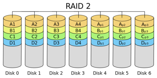
In RAID 2 (bit-level striping with dedicated Hamming-code parity), all disk spindle rotation is synchronized, and data is striped such that each sequential bit is on a different drive. Hamming-code parity is calculated across corresponding bits and stored on at least one parity drive. This theoretical RAID level is not used in practice. You need two groups of disks. One group of disks are used to write the data, another group is used to write the error correction codes. This is not used anymore. This is expensive and implementing it in a RAID controller is complex, and ECC is redundant now-a-days, as the hard disk themselves can do this themselves

  • RAID 3

RAID_3.svg

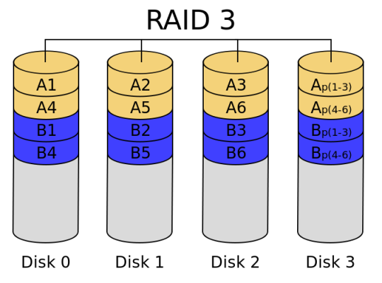
In RAID 3 (byte-level striping with dedicated parity), all disk spindle rotation is synchronized, and data is striped so each sequential byte is on a different drive. Parity is calculated across corresponding bytes and stored on a dedicated parity drive. Although implementations exist, RAID 3 is not commonly used in practice. Sequential read and write will have good performance. Random read and write will have worst performance.

  • RAID 4

675px-RAID_4.svg

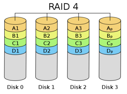
RAID 4 (block-level striping with dedicated parity) is identical to RAID 5 (see below), but confines all parity data to a single drive. In this setup, files may be distributed between multiple drives. Each drive operates independently, allowing I/O requests to be performed in parallel. However, the use of a dedicated parity drive could create a performance bottleneck; because the parity data must be written to a single, dedicated parity drive for each block of non-parity data, the overall write performance may depend a great deal on the performance of this parity drive.

  • RAID 6

RAID_6.svg

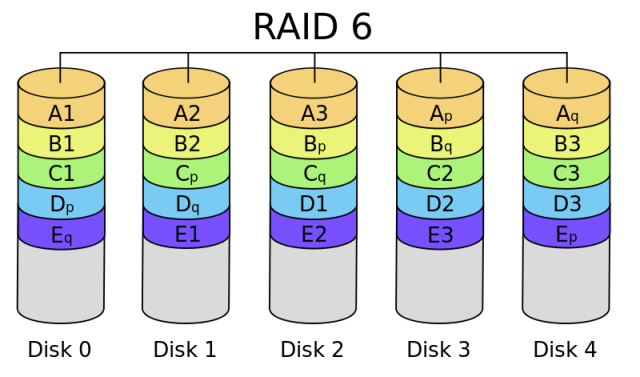
RAID 6 (block-level striping with double distributed parity) provides fault tolerance of two drive failures; the array continues to operate with up to two failed drives. This makes larger RAID groups more practical, especially for high-availability systems. This becomes increasingly important as large-capacity drives lengthen the time needed to recover from the failure of a single drive. Single-parity RAID levels are as vulnerable to data loss as a RAID 0 array until the failed drive is replaced and its data rebuilt; the larger the drive, the longer the rebuild takes. Double parity gives additional time to rebuild the array without the data being at risk if a single additional drive fails before the rebuild is complete. Like RAID 5, a single drive failure results in reduced performance of the entire array until the failed drive has been replaced and the associated data rebuilt.

Don’t use for high random write workloads

What is Parity?

Parity data is used by some RAID levels to achieve redundancy. If a drive in the array fails, remaining data on the other drives can be combined with the parity data (using the Boolean XOR function) to reconstruct the missing data.

For example, suppose two drives in a three-drive RAID 5 array contained the following data:

Drive 1: 01101101
Drive 2: 11010100

To calculate parity data for the two drives, an XOR is performed on their data:

01101101
XOR  11010100
_____________
10111001

The resulting parity data, 10111001, is then stored on Drive 3.

Should any of the three drives fail, the contents of the failed drive can be reconstructed on a replacement drive by subjecting the data from the remaining drives to the same XOR operation. If Drive 2 were to fail, its data could be rebuilt using the XOR results of the contents of the two remaining drives, Drive 1 and Drive 3:

Drive 1: 01101101
Drive 3: 10111001

as follows:

10111001
XOR  01101101
_____________
11010100

The result of that XOR calculation yields Drive 2’s contents. 11010100 is then stored on Drive 2, fully repairing the array. This same XOR concept applies similarly to larger arrays, using any number of disks. In the case of a RAID 3 array of 12 drives, 11 drives participate in the XOR calculation shown above and yield a value that is then stored on the dedicated parity drive.

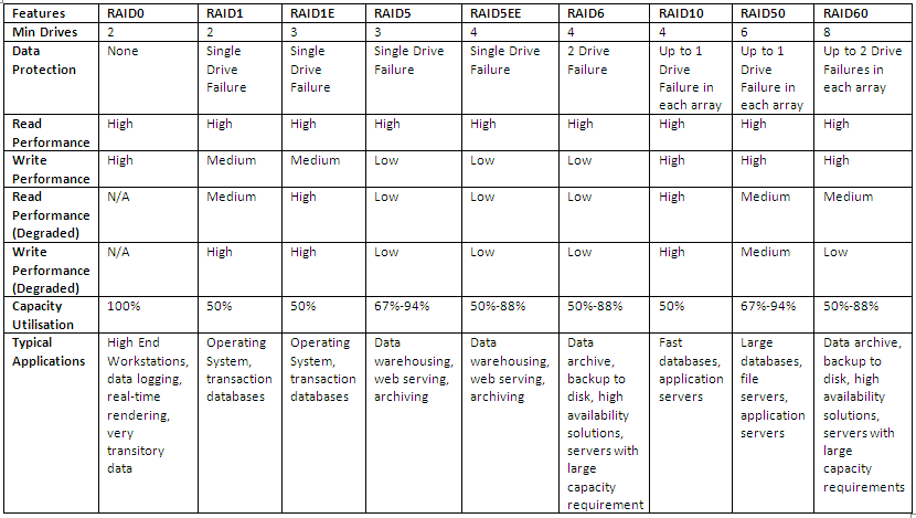
RAID Level Comparison

RAID

Interesting Link

http://www.miracleas.com/BAARF/RAID5_versus_RAID10.txt


IBM Comprestimator

What is the Comprestimator?

Comprestimator is a command line host-based utility that can be used to estimate
expected compression rate for block-devices. The Comprestimator utility uses
advanced mathematical and statistical formulas to perform the sampling and
analysis process in a very short and efficient way. The utility also displays its
accuracy level by showing the maximum error range of the results achieved based
on the formulas it uses. The utility runs on a host that has access to the devices
that will be analyzed, and performs only read operations so it has no effect
whatsoever on the data stored on the device. The following section provides
useful information on installing Comprestimator on a host and using it to analyze
devices on that host. Depending on the environment configuration, in many cases
Comprestimator will be used on more than one host, in order to analyze
additional data types.

It is important to understand block-device behavior when analyzing traditional
(fully-allocated) volumes. Traditional volumes that were created without initially
zeroing the device may contain traces of old data in the block-device level. Such
data will not be accessible or viewable in the file-system level. When using
Comprestimator to analyze such volumes, the expected compression results will
reflect the compression rate that will be achieved for all the data in the blockdevice
level, including the traces of old data. This simulates the volume mirroring
process of the analyzed device into a compressed volume. Later, when volume
mirroring is actually used to compress the data on the storage system, it will
process all data on the device (including both active data and traces of old data)
and get it compressed. After that when storing more active data on the
compressed volume, traces of old data will start getting deleted by new data that
is written into the volume. As more active data accumulates in the device the
compression rate achieved will be adjusted to reflect the accurate savings
achieved for the active data. This block-device behavior is limited to traditional
volumes and will not occur when analyzing thinly provisioned volumes

Regardless of the type of block-device being scanned, it is also important to
understand a few characteristics of common file-systems space management.
When files are deleted from a file-system, the space they occupied before being
deleted will be freed and available to the file-system even though the data on disk
was not actually deleted but rather the file-system index and pointers were
updated to reflect this change. When using Comprestimator to analyze a block-device used by a file-system – all underlying data in the device will be analyzed, regardless of whether this data belongs to files that were already deleted from the file-system. For example – you can fill a 100GB file-system and make it 100% used, then delete all the files in the file-system making it 0% used. When scanning the block-device used for storing the file-system in this example, Comprestimator (or any other utility for that matter) will access the data that belongs to the files that were already deleted.

In order to reduce the impact of block-device and file-system behavior mentioned above it is highly recommended to use Comprestimator to analyze volumes that contain as much active data as possible rather than volumes that are mostly empty of data. This increases accuracy level and reduces the risk of analyzing old data that is already deleted but may still have traces on the device.

Your primary resource for sizing and implementing: Real-time Compression in SAN Volume Controller and Storwize V7000 Redpaper

http://www.redbooks.ibm.com/Redbooks.nsf/RedpieceAbstracts/redp4859.html?Open

Instructions on how to set up IBM Real-time Compression for 45 Day Evaluation Real-time Compression Evaluation User Guide

http://www.ibm.com/support/docview.wss?uid=ssg1S7003988

Compatibility

  • Red Hat Enterprise Linux Version 5 (64-bit)
  • ESXi 5.0
  • AIX V6.1, V7.1
  • Windows 2003 Server, Windows 2008 Server (32-bit and 64-bit

Instructions for use with ESX

  • Download the installer and you should see the following zip file containing the below folders

  • Click on the Host > Configuration > Security Profile > Properties > Select Remote Tech Support > Click Options > Start > This will enable you to connect to the host remotely using Putty and WinSCP
  • Copy the installer to the server you want to run WinSCP and Putty on and make sure it is unzipped
  • Log into the host using Winscp and copy across the Comprestimator_Linux to the /tmp folder on the host
  • Next Putty into the host and login
  • Run the following command to get the list of devices
  • esxcli corestorage device list | grep dev

  • Type cd tmp to get to the diretcory you copied the Comprestimator_Linux Tool into
  • Type ./comprestimator_linux -d /vmfs/devices/disks/naa.60050768028080befc00000000000034 -p 10 -P -e -h -c outputfile -v
  • Type ./comprestimator_linux -d /vmfs/volumes/099b2072-7bd8dac0-7c5c-015dcc8bfc70 -p 10 -P -h -e -c outputfile -v
  • Type ./comprestimator_linux -d /vmware/volumes/-p 10 -P -h -e -c outputfle -v

  • Run this tool for each device


Whats the difference between SAS, Nearline SAS and SATA?

Types of Disk

When you buy a server or storage array these days, you often have the choice between three different kinds of hard drives:

  • Serial Attached SCSI (SAS)
  • Near Line SAS (NL-SAS)
  • Serial ATA (SATA).

SAS

Also known as Tier-1, these 10K & 15K RPM SAS drives provide the online enterprise performance and availability needed for mission critical application

  • General Standard in storage these days
  • Most reliable
  • Generally high performing
  • Lower BER (Bit Error Rate) than other types of disk.1 in 10^16 bits
  • SAS disks have a mean time between failure of 1.6 million hours compared to 1.2 million hours for SATA
  • SAS disks/controller pairs also have a multitude of additional commands that control the disks and that make SAS a more efficient choice than SATA.

Nearline SAS?

An NL-SAS disk is a bunch of spinning SATA platters with the native command set of SAS. While these disks will never perform as well as SAS thanks to their lower rotational rate, they do provide all of the enterprise features that come with SAS, including enterprise command queuing, concurrent data channels, and multiple host support.

  • NL-SAS drives are enterprise SATA drives with a SAS interface, head, media, and rotational speed of traditional enterprise-class SATA drives with the fully capable SAS interface typical for classic SAS drives.”
  • Same speed really as SATA. While these disks will never perform as well as SAS thanks to their lower rotational rate, they do provide all of the enterprise features that come with SAS
  • Good if you need 1TB drives in a SAS server, say for backups.
  • Not good for first or primary storage in a SAS based server.
  • Enterprise/tagged command queuing. Simultaneously coordinates multiple sets of storage instructions by reordering them at the storage controller level so that they’re delivered to the disk in an efficient way.
  • Concurrent data channels. SAS includes multiple full-duplex data channels, which provides for faster throughout of data.
  • Multiple host support. A single SAS disk can be controlled by multiple hosts without need of an expander.
  • The BER is generally 1 in 10^15 bits.
  • NL-SAS disks rotate at speeds of 7200 RPM… the same as most SATA disks, although there are some SATA drives that operate at 10K RPM.

SATA

Also known as Tier-2: these Nearline, Business Critical 5.4K and 7.2K RPM drives combine specific design and manufacturing processes for hard drives rated at 24x7x365 operations for true enterprise duty cycles. The main emphasis is on an exceptional dollars/GigaByte advantage over Tier 1 storage

  • It doesn’t perform as well as SAS and doesn’t have some of the enterprise benefits of NL-SAS
  • Used for large cheap capacity over performance

RAID Calculator

http://www.ibeast.com/content/tools/RaidCalc/RaidCalc.asp

VMware RDMs

What is RAW Device Mapping?

A Raw Device Mapping allows a special file in a VMFS volume to act as a proxy for a raw device. The mapping file contains metadata used to manage and redirect disk accesses to the physical device. The mapping file gives you some of the advantages of a virtual disk in the VMFS file system, while keeping some advantages of direct access to physical device characteristics. In effect it merges VMFS manageability with raw device access

A raw device mapping is effectively a symbolic link from a VMFS to a raw LUN. This makes LUNs appear as files in a VMFS volume. The mapping file, not the raw LUN is referenced in the virtual machine configuration. The mapping file contains a reference to the raw LUN.

Note that raw device mapping requires the mapped device to be a whole LUN; mapping to a partition only is not supported.

Uses for RDM’s

  • Use RDMs when VMFS virtual disk would become too large to effectively manage.

For example, When a VM needs a partition that is greater than the VMFS 2 TB limit is a reason to use an RDM. Large file servers, if you choose to encapsulate them as a VM, are a prime example. Perhaps a data warehouse application would be another. Alongside this, the time it would take to move a vmdk larger than this would be significant.

  • Use RDMs to leverage native SAN tools

SAN snapshots, direct backups, performance monitoring, and SAN management are all possible reasons to consider RDMs. Native SAN tools can snapshot the LUN and move the data about at a much quicker rate.

  • Use RDMs for virtualized MSCS Clusters

Actually, this is not a choice. Microsoft Clustering Services (MSCS) running on VMware VI require RDMs. Clustering VMs across ESX hosts is still commonly used when consolidating hardware to VI. VMware now recommends that cluster data and quorum disks be configured as raw device mappings rather than as files on shared VMFS

Terminology

The following terms are used in this document or related documentation:

  • Raw Disk — A disk volume accessed by a virtual machine as an alternative to a virtual disk file; it may or may not be accessed via a mapping file.
  • Raw Device — Any SCSI device accessed via a mapping file. For ESX Server 2.5, only disk devices are supported.
  • Raw LUN — A logical disk volume located in a SAN.
  • LUN — Acronym for a logical unit number.
  • Mapping File — A VMFS file containing metadata used to map and manage a raw device.
  • Mapping — An abbreviated term for a raw device mapping.
  • Mapped Device — A raw device managed by a mapping file.
  • Metadata File — A mapping file.
  • Compatibility Mode — The virtualization type used for SCSI device access (physical or virtual).
  • SAN — Acronym for a storage area network.
  • VMFS — A high-performance file system used by VMware ESX Server.

Compatibility Modes

Physical Mode RDMs

  • Useful if you are using SAN-aware applications in the virtual machine
  • Useful to run SCSI target based software
  • Physical mode is useful to run SAN management agents or other SCSI target based software in the virtual machine
  • Physical mode for the RDM specifies minimal SCSI virtualization of the mapped device, allowing the greatest flexibility for SAN management software. In physical mode, the VMkernel passes all SCSI commands to the device, with one exception: the REPORT LUNs command is virtualized, so that the VMkernel can isolate the LUN for the owning virtual machine. Otherwise, all physical characteristics of the underlying hardware are exposed.

Virtual Mode RDMs

  • Advanced file locking for data protection
  • VMware Snapshots
  • Allows for cloning
  • Redo logs for streamlining development processes
  • More portable across storage hardware, presenting the same behavior as a virtual disk file

Setting up RDMs

  •  Right click on the Virtual Machine and select Edit Settings
  • Under the Hardware Tab, click Add
  • Select Hard Disk
  • Click Next
  • Click Raw Device Mapping

If the option is greyed out, please check the following.

http://kb.vmware.com/RDM Greyed Out

  • From the list of SAN disks or LUNs, select a raw LUN for your virtual machine to access directly.
  • Select a datastore for the RDM mapping file. You can place the RDM file on the same datastore where your virtual machine configuration file resides,
    or select a different datastore.
  • Select a compatibility mode. Physical or Virtual
  • Select a virtual device node
  • Click Next.
  • In the Ready to Complete New Virtual Machine page, review your selections.
  • Click Finish to complete your virtual machine.

Note: To use vMotion for virtual machines with enabled NPIV, make sure that the RDM files of the virtual machines are located on the same datastore. You cannot perform Storage vMotion or vMotion between datastores when NPIV is enabled.

IOPs

When planning for storage to your VMware architecture, it is easy to focus on the storage capacity dimension rather than focusing on availability and performance

Capacity is generally not the limit for proper storage configurations. Capacity reducing techniques such as deduplication, thin provisioning and compression means you can now use disk capacity far more efficiently than before.

So what are IOP’s?

IOPS (Input/Output Operations Per Second, pronounced eye-ops) are a common performance measurement used to benchmark computer storage devices like hard disk drives (HDD), solid state drives (SSD), and storage area networks (SAN). As with any benchmark, IOPS numbers published by storage device manufacturers do not guarantee real-world application performance

IOPS can be measured with applications, such as Iometer (originally developed by Intel), as well as IOzone and FIO and is primarily used with servers to find the best storage configuration.

The specific number of IOPS possible in any system configuration will vary greatly, depending upon the variables the tester enters into the program, including the balance of read and write operations, the mix of sequential and random access patterns, the number of worker threads and queue depth, as well as the data block sizes.There are other factors which can also affect the IOPS results including the system setup, storage drivers, OS background operations, etc. Also, when testing SSDs in particular, there are preconditioning considerations that must be taken into account.

Computer IOP’s

Virtual Desktops use 5-20 IOP’s

Light Servers use 50-100 IOP’s

Heavy Servers – Require independent measurement for true accuracy

Storage Drive IOP’s

Enterprise Flash Drives = 1000 IOP’s pr drive

FC 15K RPM SAS Drives = 180 IOP’s per drive

FC 10K RPM SAS Drives = 120 IOP’s per drive

10K RPM SATA Drives = 125-150 IOP’s per drive

7K RPM SATA Drives = 75-100 IOP’s per drive

5.4K RPM SATA Drives = 80 IOPS per drive

Performance Characteristics

The most common performance characteristics measured are sequential and random operations.

  • Sequential operations access locations on the storage device in a contiguous manner and are generally associated with large data transfer sizes, e.g. 128 KB.
  • Random operations access locations on the storage device in a non-contiguous manner and are generally associated with small data transfer sizes, e.g. 4 KB.

Useful Performance Link

http://kb.vmware.com/selfservice/microsites/search.do?language=en_US&cmd=displayKC&externalId=1031773